hedging strategies using binary options

Option Greeks and Hedging Strategies                          
The aims of the actual research are, firstly, to present some of the near efficient methods to hedge selection positions and, secondly, to show how important pick Greeks are in volatility trading. Information technology is worth mentioning that the present written report has been completely developed by Liying Zhao (Quantitative Analyst at          HyperVolatility) and all the simulations accept been performed via the          HyperVolatility Option Tool–Box.          If you are interested in learning about the fundamentals of the various option Greeks please read the following studies          Options Greeks: Delta, Gamma, Vega, Theta, Rho          and          Options Greeks: Vanna, Amuse, Vomma, DvegaDtime          .
In this research, we will assume that the implied volatilityσis not stochastic, which means that volatility is neither a part of fourth dimension nor a part of the underlying cost. Every bit a practical affair, this is not true, since volatility constantly change over fourth dimension and tin can inappreciably be explicitly forecasted. Nonetheless, doing researches under the static–volatility framework, namely, the Generalized Black–Scholes–Merton (GBSM) framework, we tin can hands grasp the bones theories and and so naturally extend them to stochastic volatility models.
Recall that the Generalized Black–Scholes–Merton formula for pricing European options is:
                      C = Se (b-r)T N(d1) — Xe -rT Northward(d2)                  
                      P = Xe -rT North(–d2) — Se (b-r)T N(–d1)                  
Where
                      
                      
And          N (          )          is the cumulative distribution role of the univariate standard normal distribution.          C          = Phone call Price,          P          = Put Price,          Due south          = Underlying Cost,          X          = Strike Price,          T          = Fourth dimension to Maturity,          r          = Run a risk–complimentary Involvement Charge per unit,          b          = Cost of Carry Rate, σ= Implied Volatility.
Accordingly, start club GBSM option Greeks can be divers as sensitivities of the option price to one unit change in the input variables. Consequentially, 2nd or 3rd–order Greeks are the sensitivities of first or second–order Greeks to unit of measurement movements in diverse inputs. They can also exist treated every bit various dimensions of adventure exposures in an option position.
          one. Risk Exposures        
Differently from other papers on volatility trading, nosotros will initially look at the Vega exposure of an selection position.
          1.1 Vega Exposure        
Some of the variables in the selection pricing formula, including the underlying cost          South,          chance–free interest rate          r          and cost of carry charge per unit          b, tin can exist directly nerveless from market sources. Strike price          X          and time to maturity          T          are agreed with the counterparties. Still, the implied volatility σ, which is the market expectation towards the magnitude of the future underlying cost fluctuations, cannot be explicitly derived from any market source. Hence, a number of trading opportunities arise. Likewise directional trading, if a trader believes that the future volatility will ascension she should buy it while, if she has a downward bias on future volatility, she should sell information technology. How can a trader buy or sell volatility?
We already know that Vega measures option'southward sensitivity to small movements in the implied volatility and it is identical and positive for both telephone call and put options, therefore, a rise in volatility volition atomic number 82 to an increment in the option value and          vice versa. Equally a result, options on the same underlying asset with the same strike price and expiry date may be priced differently by each trader since everyone tin input her ain implied volatility into the BSM pricing formula. Therefore, trading volatility could be, for simplicity, achieved by simply ownership nether–priced or selling over–priced options. For finding out if your unsaid volatility is college or lower than the market one, y'all can refer to          this research                    that we previously posted.
Let's presume an pick trader is holding a so–called 'naked' short option position, where she has sold 1,000 out–of–the–money (OTM) phone call options priced with          Southward=$ninety,          10=$100,          T=30 days,          r=0.5%,          b=0, σ=30%, which is currently valued at $434.3. Suppose the marketplace agreed implied volatility decreases to 20%, other things beingness equal, the option position is at present valued at $70.6. Clearly, there is a marking–to–market turn a profit of $363.seven (434.3–70.6) for this trader. This is a typical example of Vega exposure.
          Figure 1          shows the Vega exposure of higher up the option position. It tin be easily observed that the Vega exposure may augment or erode the position value in a not–linear manner:
                          
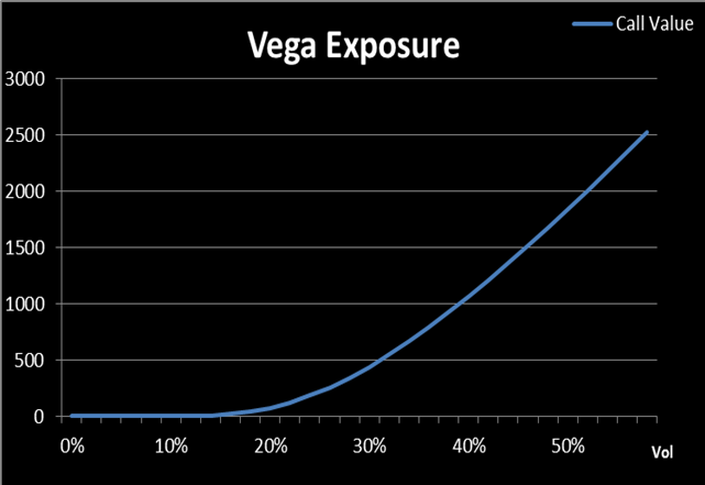
          (Effigy 1. Source:          HyperVolatility Option Tool — Box)        
A trader can achieve a given Vega exposure by buying or selling options and can brand a profit from a better volatility forecast. However, the value of an option is not affected solely by the implied volatility because when exposed to Vega risk, the trader will simultaneously exist exposed to other types of risks.
          i.2 Theta Exposure        
Theta is the alter in selection toll with respect to the passage of time. It is likewise called 'fourth dimension decay' because Theta is considered to be 'always' negative for long pick positions. Given that all other variables are constants, option value declines over time, so Theta tin be generally referred to equally the 'price' ane has to pay when buying options or the 'reward' i receives from selling options. However, this is not ever true. Information technology is worth noting that          some researchers have reported that Theta can be positive for deep ITM put options on not–dividend–paying stocks. Even so, co-ordinate to our enquiry, which is displayed in          Effigy 2, where          Ten=$100,          T=30 days,          r=0.five%,          b=0, σ =30%, the status for positive Theta is non that rigorous:
                          
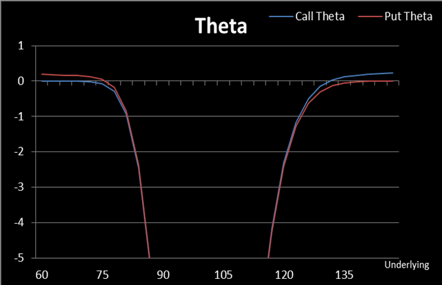
          (Figure ii. Source:          HyperVolatility Choice Tool — Box)        
For deep in–the–money (ITM) options (with no other restrictions) Theta can exist slightly greater than 0. In this example, Theta cannot be called 'time disuse' any longer because the time passage, instead, adds value to bought options. This could be thought of as the bounty for choice buyers who decide to 'requite up' the opportunity to invest the premiums in risk–free assets.
Regarding the same example, if an choice trader has sold 1,000 OTM telephone call options priced with          Southward=$90,          X=$100,          T=30 days,          r=0.v%,          b=0, σ=thirty%, the Theta exposure of her option position will be shaped like in          Figure 3:
                          
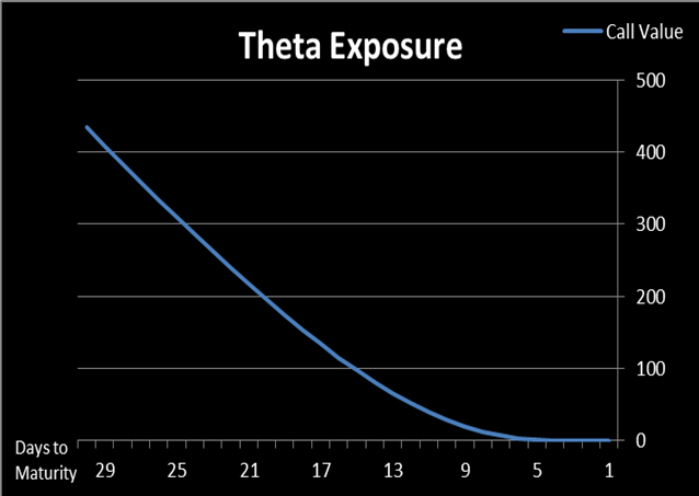
          (Figure 3. Source:          HyperVolatility Selection Tool — Box)        
In the real globe, none can stop fourth dimension from elapsing then Theta gamble is foreseeable and can inappreciably exist neutralized. We should take Theta exposure into business relationship but do not need to hedge it.
          1.3 Involvement Rate/Cost of Carry Exposure (Rho/Price of Conduct Rho)        
The cost of acquit rate          b          is equal to 0 for options on commodity futures and equals          r–q          for options on other underlying assets (for currency options,          r          is the chance–free involvement charge per unit of the domestic currency while          q          is the foreign currency'south involvement rate; for stock options,          r          is the take a chance–gratuitous involvement rate and          q          is the proportional dividend charge per unit). The being of          r,          q          and          b          does accept an influence on the value of the option. However, these variables are relatively determinated in a given period of time and their change in value has rather insignificant effects on the option price. Consequently, we volition not become too deep into these parameters.
          1.4 Delta Exposure        
Delta is the sensitivity of the pick cost with regard to changes in the underlying price. If we recall the aforementioned scenario (where a trader has sold 1,000 OTM call options priced with          S=$ninety,          X=$100,          T=xxx days,          r=0.5%,          b=0, σ =30%, valued at $434.3) if the underlying price moves downwards, the position tin still be able to make profits because the options will have no intrinsic value and the seller can go along the premiums. Even so, if the underlying asset is traded at, say, $105, all other things being equal, the choice value becomes $vi,563.7, which leads to a notable mark–to–market loss of $6,129.iv (6,563.7–434.3) for the option writer. This is a typical example of Delta risk one has to face when trading volatility.          Effigy four          depicts the Delta exposure of the above mentioned option position, where we tin can run into that the change in the underlying asset price has pregnant influences on the value of an option position:
                          
          (Figure iv. Source:          HyperVolatility Option Tool — Box)        
Compared to Theta, Rho and toll of acquit exposures, Delta risk is definitely much more dominating in volatility trading and it should exist hedged in order to isolate volatility exposure. Consequentially, the residuum of this paper volition focus on the introduction to various approaches for hedging the adventure with respect to the movements of the underlying price.
          2. Hedging Methods        
At the beginning of this department, we should clearly define 2 confusable terms: hedging costs and transaction costs. Generally, hedging costs could consist of transaction costs and the losses caused by 'purchase high' and 'sell depression' transactions. Transaction costs can exist broken down into commissions (paid to brokers,          etc.) and the bid/ask spread. These two terms are usually confounded because both of them have positive relationships with hedging frequency. Mixing these two terms up may be acceptable, but we should proceed them articulate in listen.
          two.i 'Covered' Positions        
A 'covered' position is a static hedging method. To illustrate information technology, let us assume that an option trader has sold 1,000 OTM call options priced with          S=$90,          X=$100,          T=thirty days,          r=0.v%,          b=0, σ=30%, and has gained $434.three premium. Compared to the 'naked' position, this time, these options are sold simultaneously with some purchased underlying assets, say, 1,000 stocks at $xc. In this case, if the stock price increases to a value above strike price (due east.g.          $105) at maturity, the counterparty will have the motivation to practise these options at $100. Since the option writer has enough amount of stocks on manus to meet the do need, ignoring any commission, she can even so get a net turn a profit of one,000*(100–90) + 434.three= $x,434.iii. On the reverse, if the stock price stays under the strike cost (e.g.          $85) upon decease date, the seller'southward premium is safe but has to suffer a loss in stock position which in full makes the trader a negative 'profit' of i,000*(85–90) + 434.4=-$4565.seven. The 'covered' position tin offering some degrees of protection just too induces extra risks in the concurrently. Thus, it is non a desirable hedging method.
          two.2 'Stop-Loss' Strategy        
To avoid the risks incurred by stock prices' downwardly trends in the previous case the option seller could defer the buy of stocks and monitor the movements of the stock market. If the stock price is higher than the strike toll, i,000 stocks will be bought as soon as possible and the trader will keep this position until the stock toll will fall below the strike. This strategy seems like a combination of a 'covered' position and a 'naked' position, where the trader is 'naked' when the position is safe and he is 'covered' when the position is risky.
The 'stop-loss' strategy provides some degrees of guarantee for the trader to make profits from option position, regardless of the movements of the stock cost. However, in reality, since this strategy involves 'buy high' and 'sell depression' types of transactions, it can induce considerable hedging costs if the stock price fluctuates around the strike.
          2.three Delta–Hedging        
A smarter method to hedge the risks from the movements of the underlying price is to directly link the amount of bought (sold) underlying nugget to the Delta value of the option position in order to form a Delta– neutral portfolio. This approach is referred to as Delta hedging. How to fix a Delta–neutral position?
Once again, if a trader has sold one,000 telephone call options priced with          Due south=$90,          X=$100,          T=30 days,          r=0.five%,          b=0, σ=thirty% the Delta of her position volition be -$119 (-one,000*0.119), which means that if the underlying increases past $ane, the value of this position will appropriately decrease by $119. In guild to starting time this loss, the trader tin can buy 119 units of underlying, say, stocks. This stock position will give the trader $119 turn a profit if the underlying increases by $ane. On the other hand, if the stock price decreases past $i, the loss on the stock position will then be covered by the proceeds in the option position. This combined position seems to brand the trader immunized to the movements of the underlying toll.
However, in the example the underlying trades at $91, we can estimate that the new position Delta will be -$146. Obviously, 119 units of stocks can no longer offer full protection to the option position. As a result, the trader should rebalance her position by buying 27 more stocks to brand it Delta–neutral again.
Past doing this continuously, the trader can have her option position well protected and will savour the profit deriving from an improved volatility forecasting. Nevertheless, it should be noted that Delta–hedging too involves 'buy high' and 'sell low' operations which could cause a loss for every transaction related to the stock position. If the price of the underlying is considerably volatile, the Delta of the option position would change frequently, pregnant the option trader has to adjust her stock position appropriately with a very high frequency. Every bit a upshot, the cumulative hedging costs can reach an unaffordable level inside a short menstruation of time.
The aforementioned example show that increasing hedge frequency is effective for eliminating Delta exposure merely counterproductive equally long as hedging costs are concerned. To reach a compromise betwixt hedge frequency and hedging costs, the following strategies tin can be taken into considerations.
          2.four Delta–Gamma Hedging        
In the last section, we take found that Delta hedging needs to be rebalanced along with the movements of the underlying. In fact, if nosotros tin can make our Delta allowed to changes in the underlying price, we would not need to re–hedge. Gamma hedging techniques tin help the states accomplishing this goal (recall that Gamma is the speed at which the Delta changes with respect to movements in the underlying price).
The previously reported example, where a trader has sold 1,000 telephone call options priced with S=$ninety,X=$100,T=30days,r=0.5%,b=0            ,        
σ          =xxx% had a position Delta equal to -$119 and a Gamma of -$26. In lodge to brand this position Gamma–neutral, the trader needs to buy some options that can offer a Gamma of $26. This can be easily washed by buying one,000 phone call or put options priced with the same parameters equally the sold options. All the same, buying i,000 call options would erode all the premiums the trader has gained while ownership 1,000 put options would cost the trader more, since put options would be much more expensive in this case. A positive internet premium can be achieved by finding some cheaper options.
Let united states assume that the trader has decided to choose, equally a hedging tool, the call option priced with          S=$90,          Ten=$110,          T=30 days,          r=0.5%,          b=0, σ=xxx%, with 0.011 Delta and 0.00374 Gamma. To offset his sold Gamma, the trader needs to buy 26/0.00374 = 6,952 units of this choice which toll him $197.3 which leads to an actress Delta of six,952*0.011=$76. At this point, the trader has a Gamma–neutral position with a cyberspace premium of $237 (434.three–197.3) and a new Delta of -$43(-119+76). Therefore, ownership 43 units of underlying will provide the trader with Delta neutrality. Now, let's suppose that the underlying trades at $91, the Delta of this position would become -$32 only since the trader had already purchased 43 units of stocks, she only needs to sell 12 units to brand this position Delta–neutral. This is definitely a better do than buying 27 units of stocks as explained in department 2.3 where the trader had only Delta neutralized but was however running a non–zero Gamma position.
However, Delta–Gamma Hedging is not as adept as we expected. In order to explain this, let us look at            Figure-5          which shows the Gamma curve for an option with          Southward=$90,          X=$110,          T=xxx days,          r=0.five%,          b=0, σ=30%:
                          
          (Effigy 5. Source:          HyperVolatility Selection Tool — Box)        
We can see that Gamma is also changing along with the underlying. As the underlying comes closer to $91, Gamma increases to 0.01531 (it was 0.00374 when the underlying was at $90) which means that, at this point, the trader would need $107 (6,954*0.01531) Gamma and not $26 to offset her Gamma risk. Hence, she would take to buy more options. In other words, Gamma–hedging needs to be rebalanced every bit much as delta — hedging.
Delta–Gamma Hedging cannot offer full protection to the option position, but it can be deemed equally a correction of the Delta–hedging fault because information technology can reduce the size of each re–hedge and thus minimize costs.
From section 2.3 and 2.four, we tin can conclude that if Gamma is very modest, we can solely utilize Delta hedging,          or else we could adopt Delta–Gamma hedging. However, we should bear in mind that Delta–Gamma hedging is good only when Speed is minor. Speed is the curvature of Gamma in terms of underlying toll, which is shown in Figure — 6:
                          
          (Effigy six. Source:          HyperVolatility Pick Tool — Box)        
Using the bones knowledge of Calculus or Taylor's Series Expansion, nosotros can evidence that:
                      Δ Option Value ≈ Delta * ΔS + ½ Gamma * ΔS + 1/vi Speed * ΔS                  
We tin can see that Delta hedging is skilful if Gamma and Speed are negligible while Delta–Gamma hedging is meliorate when Speed is small plenty. If whatsoever of the terminal two terms is meaning, we should seek to find other hedging methods.
          2.5 Hedging Based on Underlying Price Changes / Regular Fourth dimension Intervals        
To avert infinite hedging costs, a trader can rebalance her Delta after the underlying price has moved by a certain amount. This method is based on the noesis that the Delta risk in an option position is due to the underlying movements.
Some other alternative to avoid over–frequent Delta hedging is to hedge at regular time intervals, where hedging frequency is reduced to a fixed level. This approach is sometimes employed past big financial institutions that may take option positions in several hundred underlying assets.
However, both the suitable 'underlying cost changes' and 'regular time intervals' are relatively capricious. Nosotros know that choosing good values for these 2 parameters is of import but so far we have not institute any good method to observe them.
          two.vi Hedging by a Delta Band        
There be more than advanced strategies involving hedging strategies based on Delta bands. They are effective for finding the best trade–off betwixt risks and costs. Among those strategies, the Zakamouline band is the about feasible one. The Zakamouline band hedging dominion is quite unproblematic: when the Delta of our position moves exterior of the band, we need to re–hedge and just pull it back to the edge of the band. Still, the theory backside it and the derivation of it are not elementary. Nosotros are going to accost these issues in the next research report.
          Effigy-7          provides an instance of the Zakamouline bands for hedging a short position consisting of one,000 European call options priced with          S=$90,          X=$110,          T=30 days, r=0.5%,          b=0, σ=thirty%:
                          
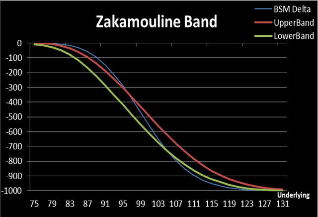
          (Figure 7. Source:          HyperVolatility Pick Tool — Box)        
In the next report, we will see how the Zakamouline band is derived, how to implement it, and volition also run across the comparison of Zakamouline band to other Delta bands in a quantitative manner.
The          HyperVolatility Forecast Service          enables you to receive statistical analysis and projections for 3 nugget classes of your choice on a weekly ground. Every member can select up to 3 markets from the following list: E-Mini S&P500 futures, WTI Crude Oil futures, Euro futures, VIX Alphabetize, Gold futures, DAX futures, Treasury Bond futures, High german Bund futures, Japanese Yen futures and FTSE/MIB futures.
Send us an e-mail at          info@hypervolatility.com                    with the list of the iii asset classes y'all would like to receive the projections for and nosotros volition guarantee you a 14 day trial